Code cells

Each code cell is a notebook-style overlay anchored to a point on the board. It has a writable Python editor (Tab indents; Ctrl/Shift+Enter runs) and an output area. A grip on the bottom-right corner resizes it to any width and height; once sized, the box scrolls internally instead of auto-growing, and a draggable divider between the editor and the output lets you rebalance the two. The chosen size and split persist.

Code or Markdown

A cell-type dropdown in the header (beside Run) switches a cell between Code and Markdown in place, notebook-style. Switching keeps the cell’s id, parent link, source, and size — so children stay linked and the layout is unchanged. A Markdown cell renders its source as Markdown instead of running it; double-click the preview to re-edit.

Running code

• ▶ Run executes just this cell.
• ▶▶ fast-forwards: runs this cell and every cell below it.
• 🪄 Magic wand asks the configured LLM to write, fix, or improve the cell and streams the result straight into the editor, replacing what was there. The prompt is built from the current source plus the last run’s traceback if it errored — and a #> comment is treated as a targeted instruction to apply. If there’s no LLM configured (or the request fails) the original code is restored and the reason is shown in the output.
• ⭳ exports the cell’s lineage (root → this cell) as a .ipynb notebook.

A notebook-style execution count appears in the header: [ ] unrun, [*] running, [n] run.

Rich output: stdout/stderr stream live, and the final expression renders as the richest representation available — matplotlib figures and PNGs as images, pandas DataFrames / HTML as tables, SVG — falling back to text.

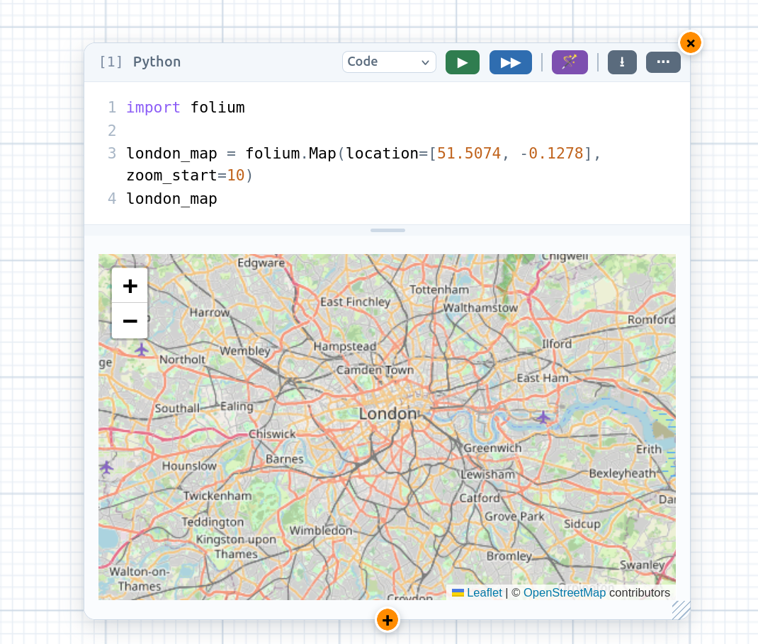
A cell’s rendered output is saved with the board and restored on reload without re-running, and when you’re signed in it’s shared with collaborators too (execution itself stays local — each person runs their own kernel). The one exception is live interactive widgets, which need a running kernel and reappear only after you re-run the cell.

The kernel

• The default kernel runs Python compiled to WebAssembly, entirely in your browser — loaded lazily and preloaded when you create your first cell. A status pill (top-right) shows loading / ready / running. Common packages like numpy, pandas, and matplotlib auto-load on import.
• Some pure-Python packages that aren’t in the default distribution install from PyPI on first import — currently folium (interactive maps), ipycanvas, and ipywidgets — with the status pill showing Installing ….
• Interactive widgets: import ipywidgets gives you live sliders, buttons, interact, Output, etc., rendered as standard interactive widget views and fully interactive (callbacks run and push values back into Python). Because widgets are live kernel objects they aren’t saved — a restored or shared cell shows its widgets only after you re-run it.
• A remote server kernel backend is also wired up if you’d rather run against a real kernel.

Calling the model from Python

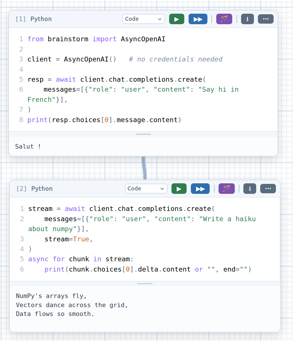
Code cells can talk to the same model you’ve configured for chat — with no API keys in your notebook. Import the built-in client and call it with the OpenAI Chat Completions API you already know:

from brainstorm import AsyncOpenAI

client = AsyncOpenAI()   # no credentials needed

resp = await client.chat.completions.create(
    messages=[{"role": "user", "content": "Say hi in French"}],
)
print(resp.choices[0].message.content)

• No credentials. Which model runs — and whether it’s billed — follows the Chat track in the Models tab: your own key (free, local) or a hosted model against your balance. The cell never sees a key, so hosted calls from code are metered exactly like chat, and BYOK calls stay on your machine.

• Top-level await. Cells run asynchronously, so you await calls directly. The client is async — AsyncOpenAI, also importable as openai for drop-in snippets.

• Streaming renders live in the output as tokens arrive:

  stream = await client.chat.completions.create(
      messages=[{"role": "user", "content": "Write a haiku about numpy"}],
      stream=True,
  )
  async for chunk in stream:
      print(chunk.choices[0].delta.content or "", end="")
  

• OpenAI-compatible. messages, temperature, resp.choices[0].message.content, and the streaming chunk.choices[0].delta.content all behave as you’d expect. A failed request (for example an empty hosted balance) raises a catchable brainstorm.LLMError.

Combined with linked sheets and images below, this lets a cell read your data and reason over it in the same place — no separate notebook, no key management.

The cell tree

Cells form a tree — each cell has at most one parent — that chains toward running as one notebook.

• The orange + on a cell’s lower edge: click it to spawn a child cell beneath, or drag from it to wire up the tree. While dragging, a Bézier follows your pointer; drop it onto another cell to make that cell a child, or onto empty board to spawn a fresh child there.
• The drop target highlights green (valid) or red (would create a cycle — cycles are disallowed).
• Remove a link by hovering anywhere along a connector: an × appears at its midpoint; click it to detach the child (it becomes a new root).

Linked data (sheets, images, videos)

Code cells can pull in spreadsheets, images, and videos from the board as data, without any file wrangling:

• Spreadsheets. Every spreadsheet has its own orange +: click it to spawn a code cell that already reads the sheet, or drag from it onto an existing cell to link the sheet in. Before the cell runs, each linked sheet — and any inherited from an ancestor cell — is converted to .xlsx and written into the kernel, then exposed via an auto-injected SHEETS dict (name → path), so you can pd.read_excel(SHEETS["…"]).
• Images. Drag an image’s orange + onto a code cell to link it as data (a plain click still opens the transform dialog). Linked images — and any inherited from an ancestor — are written into the kernel and exposed via an auto-injected IMAGES dict (image1, image2, … → path), so you can PIL.Image.open(IMAGES["image1"]).
• Videos. Drag a video bubble’s orange + onto a code cell (or click it and pick Python to spawn a cell that already reads the clip). Linked videos — and any inherited from an ancestor — are written into the kernel and exposed via an auto-injected VIDEOS dict (video1, video2, … → path), so you can cv2.VideoCapture(VIDEOS["video1"]). A run that writes a video file surfaces it as its own connected video bubble, too.

Links show as a green connector with the same hover-to-remove ×, and the data is re-materialized on every run, so the kernel always sees the current contents. (All three work with the in-browser kernel.)

Branch execution

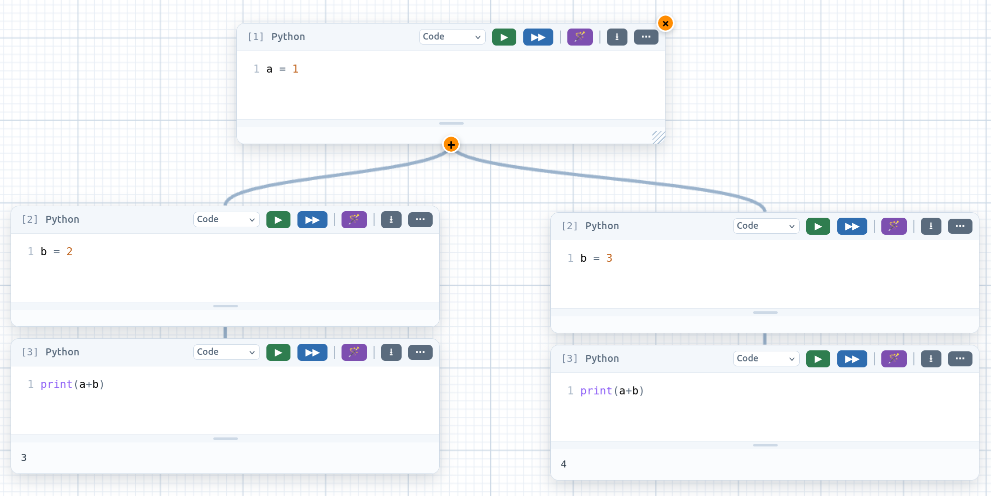
A cell can have multiple children (a branch). The semantics:

• Numbering is a cell’s depth in its tree (root = [1]). Each root→leaf path reads [1], [2], [3]…, so siblings at the same level share a number.
• ▶▶ fast-forward runs from the clicked cell downward through its subtree (it does not re-run ancestors), continuing from the live interactive kernel state. At each branch, sibling subtrees fork their own namespace so independent “what-if” branches can’t pollute each other.
• Stop-on-error halts the failing branch at the erroring cell; the remaining branches still run.
• Export captures the lineage that produced a cell (root → that cell).